The Road to BERT

A unique journey of evolution of text representation with Deep Learning

Deep Learning (DL) is about automatically learning hierarichal representations of data. So the main question in NLP is how to best represent language data (text or speech), so that to fit a certain NLP task. In this tutorial we will:

• Go through the different ways to represent language data, specifically text, and the origins of those representations linking them to the nature of the input; structured or unsturtured, and how different variable types affect our modeling decisions.

• Then we will give and overview about the Transfer learning in NLP and relate that to the breakthrough in CV with pre-trained networks on ImageNet dataset.

• This will lead us to the SoTA architecures today in NLP, like BERT, GPT, XLNet,…etc.

The tutorial focuses on the following key ideas:

• Transfer learning and Encoder-Decoder paradigm.
• Analogy between Computer Vision (CV) and NLP, leading to the so-called “ImageNet moment of NLP”.
• The symbolic nature of language, leading to words vectors.
• The sequential nature of language, versus the spatial nature of images, leading to the importance of context in NLP.

The Deep Learning way of thinking

I will start by quoting the Deep Learning (DL) definition from the Deep Learning Book by Ian Goodfellow, Yoshua Bengio, Aaron Courville:

“Deep learning is a particular kind of machine learning that achieves great power and flexibility by learning to represent the world as a _nested hierarchy of concepts, with each concept defined in relation to simpler concepts, and more abstract representations computed in terms of less abstract ones”_

From the above definition, the DL way of thinking is to transform the raw data, into a structured form, by identifying the useful features.

We don’t know ahead how many of those features we need, and how many levels of hierarichal refinement are required, and even what those features will eventually represent!. We leave the gradients lead the way, thinking of those features transforms as factors that contribute to the end goal or task.

The fact that these features are factors that lead to better achieve the task, and they are not observed (hidden inside the hierarichy of concepts), give them another name: latent features, and sometimes, latent codes.

We deal with structured and unstructured data. Although strucutured data comes usually in a tabular form, where columns can be thought of as the “features”. DL further refines those features into higher level, and derive more of those features, leading to discovering “more” structure, virtually adding more columns.

Example inspired by Andrew Ng example in AI4Everyone course on Coursera

On the other hand, unstructured don’t even have those “columns”. Images, text and speech are all unstructured data. They are just a bunch of numbers representing the input.

The above concepts are easily visualized for images from CV domain. The image below from the Deep Learning with Python book, Chapter 5, shows a high level abstraction of how the hierarichy of concepts can be understood in the context of images classificaiton.

src

Deep Learning with Python book, Chapter 5

Two important notes to be drawn from the above discussion:

1- Numerical nature of images

The basic constituents at the raw level are pixels.

The advantage is that, these pixels can now be “correlated” to each others in some vector space of “colors”, where a pixel degree of brightness is encoded with 1D vector, while colored ones with 3D vectors. All vectorial operations apply on those vectors. For example, similar colors lie near each others in that vectorial space.

2- Spatial context - higher level refinement for CV

The hierarichal aggregation of pixels, into higher level concepts as edges,..etc, is done in the spatial domain of the image. This forms a spatial context of the pixels; where nearby pixels form together some context or feature.

ConvNets are the best spatial aggregators for images. They can then further refines this raw form of strucutre in pixels, into higher level latent features, that are not directly observed from the pixels, by detecting edges, leading to constructs like corners, leading to higher level features like eyes, mouth,…etc for faces recognition tasks for example.

As stated in the beginning, the analogy between CV and NLP will lead many parts of the tutorial. Now we need to answer similar questions for NLP:

• If words are the anlogous raw consituents to pixels (sometimes characters), how to represent them?

• How to refine the raw input words/characters into higher level concepts, as we did for images?

Sequential context - higher level refinement for NLP

Unlike image data, language data usually holds a “sequential” context. Hence, the hierarichal features in case of NLP is to “aggregate” words into group of word features (called n-grams), the sentence, then documents,…etc. This happens using sequence models like RNNs or LSTMs. Later we will see other models like CNN1D and Transformers. The easiest way to visualize such sequential dependency is through parsing trees:

src

Symbolic nature of language

Language tasks (speech and text) have special characteristic. Unlike images, the basic constituents (say words) are not contineous variables, but rather symbolic or categorical variables. The mere value of the symbol does not tell anything about the data.

What do I know about your from just your name?

A name is just a “unique identifier”! It doesn’t tell much about a person. Other personal traits and characteristics does. In other words, these are the “factors” that define a person. Such factors are hidden (“latent”) when we just look at the name. A very nice example and explanation of this particular example can be found in this excellent post.

If we take this example to the world of language, and particularly words, now what we know about a word by just knowing it’s index in a vocabulary?.

Such symbolic representation, does not support any vecotrial operations. For example, we cannot measure the similarity of words in the categorical space, since every word lies on an access of a high dimensional space, or in other words, orthogonal to all other words.

This adds further challenge, to first “create” the basic raw meaning of the symbols. In other words, we want to come-up with an encoding that better represent the building blocks, like words, given their symbolic or categorical nature.

In the example above, we can set some “Weights” to how “Political” and how “Sportive” is a given word. Now we have a “Vector” representing each word. The way we create that vector is by first deciding on some “factors” that are important for us to specify a word meaning, and then giving each word a “weight” with repsect to that factor. Now, we can correlate words to each others in the new vector space.

The above discussion reveals that, even within unstructured data, the level of encoding of the raw data implies to have extra encoding of the input, before even trying to refine it in hierarichal layers like a deep neural network. This is a challenge specific to language tasks. That’s why NLP is often said to be the task of converting text into structured form, that leads to NLU+NLG

Now the questions are:

• How to decide on those factors? (which factors are important and which are not to specify a word? How many factors?)

• How to assign the weights for each factor per word?

Digression: Strucured DL

The same discussion applies to strucutured/tabular (as in the example above for the demand prediction features refinement), where categorical columns have the same requirement of extra encoding into meaningful representation, before proceeding with DL. This gives rise to a branch of DL called structured DL, which starts to grasp high attention as in the recent TF2 structured column features.

Embedding

Basically, what we need is a mapping from symbolic/categorical space, into another space. The requirement on that space shall be that: words of simialr meanings and context are near each others. In the new space, all vecotrial operations hold. This mapping is called an Embedding; a mapping from categorical to vecotrial space. Again, it’s a generic concept to all structured data.

To find this mapping, we need to transform the word symbols, into some latent factors, say n of them, that better represents it. Those n-latent factors together represent a word in an n-dim space. Each one of them is a feature or factor of the word. We won’t observe them, neither we have access control to set their values in the context of DL, that’s why they are latent.

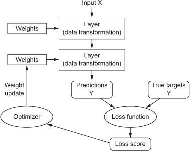
How to learn the Embeddings?

As stated earlier, an Embedding is just a mapping. In mathematics, a function is just a mapping from one space to another. So we want to find this function. The DL way of thinking is to follow parametric models framework, and approximate the function mapping with a number of parameters, or weights. Finding those weights is equivalent to finding the function. To find the values of those weights, we learn them through gradient based optimization.

src

Since our mapping is from a categorical to vector space, the function can be viewed as a table. Each symbol category has a row. The columns represent the symbol features or latent factors. So a row is just a features vector representing the symbol (say a word), sometimes refered to as latent code, and mostly known as Embedding vector. This table is called an Embedding matrix. This is better visualized as in the example above, where every word has a row, while words features are the columns (Political, Sportive,…).

In case of word vectors Embeddings, we don’t know ahead the number of latent factors, so we just set it to some number and treat this number as a hyper parameter to be set later (later we give some heauristic or rule of thumb for it).

Bag-of-words (BoW) model

A simplified model that can be used to learn Embeddings is shown below. Now, we have the Embedding table as a parametric model. To get a representation of a given word symbol, we just need to look-up its corresponding row. This look-up operation can be formulated a dot-product of a one-hot encoded (OHE) word vector, and the Embedding Matrix. The resulting word vector is the corresponding row to the word index (shown in red in the figure below). With that, we have a fully differential operation, and can now be part of any model that learns end to end usign gradient based optimization framework.

Transfer Learning in NLP

Word level TL: Pre-trained word vectors

As described above, any parametric end-to-end differentiable model can be used to learn the weights of the Embedding matrix. All text data is composed of words. Moreover, for a given language, the vocabulary of those words is similar for any task. For example, if you train your model for text classification, or machine translation, the inputs to both will be in the same space of words (vocabulary) for a given language.

This means that, the words features are universal to all tasks, and should not be task dependent. In other words, if we somehow find a universal Embedding table that represents all English words, we can use it for all tasks.

The question now is: how to find this universal Embedding table?

The answer is to employ Transfer Learning (TL). TL happens from source to target domains. For TL to be the most effective, the similarity between both domains should be as maximum as possible. By similarity it means the inputs are similar, and also the output tasks are related or relevant to each others. The more similar the two tasks, the more re-use of the transfered layers is possible. Moreover, the amount of data on which the source model is trained on should be large enough to generalize well to other tasks. In this case, even if small amount of data is avaliable for the target task, we can re-use many layers from the source model, and fine tune few new layers to match the target.

src

The idea is to find an NLP task, such that:

• This task is central and related to all other NLP tasks, such that similarity between both domains are high.

• The training of that task should be done on huge data, such that useful features are captured, and generalized to all other tasks.

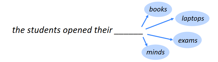
Language Models(LM)

Langauge modeling in its common form is simply to predict the next word, given a sequence of words. It can be generalized to characters (or tokens in general). Traditionaly this can be achieved in probablistic and statistical ways of modeling n-grams, which is called Staistical Language Models (SLM). Neural networks excel in this task, making Neural Langauge Models (NLM) the norm, following Bengio’s paper for NLM.

Why LM?

LM is a best fit for all the criteria to be a source task:

• It is central to almost all downstream NLP tasks. Max relevance.
• Its training is self-supervised (x=word_0, word_1,..word_N, y=word_N+1). No need of human annotation. So can be easily trained on huge corpora like wikipedia.

Language modeling tasks

The LM task can take many forms:

• Next-word prediction: predict the next word (wt), given context of words (w0..wt-1). It’s like “what is the next word”. Sequential Multi-inputs, Single output model. This is often referred to as Neural Language Models (NLM), when done using Neural Nets.

[https://miro.medium.com/max/1000/1_MrDp6w3Xc-yLuCTbco0xw.png](https://miro.medium.com/max/1000/1_MrDp6w3Xc-yLuCTbco0xw.png)

• Continous Bag of Words (CBOW): predict the Central word (wt), given context words (w0..wt-1, wt+1,….wT). It’s like “complete the missing word”. Multi-inputs, Single output model.

• Skip-gram: predict the context words (w0..wt-1, wt+1,….wT), given the cental central word (wt). Single input, Multi-outputs model.

src

Word2Vec and GloVe

The last two forms are specifically used in the famous word2vec tool. Some other ways to learn words given more global context, like documents statistics, is possible, like in GloVe.

ELMo

We need to refine a bit the concept of universal Embedding. Although the same vocabulary is used over all language tasks, however, the same word symbol holds different meaning in different contexts.

In the above Embeddings (word2vec, GloVe,…etc), the same Emebdding matrix is used, and any word has the same representation regardless of its context. In other words, a word has one, and only one, entry in the Embeddings table, no matter its context is. Accordingly, the word features (latent factors), should change according to the context. What we need is a Embedding vector, given the context.

The idea of ELMo is to build “contextualized” representations of words. ELMo uses TL from NLM using traditional next-word prediciton task. It uses a Bi-directional LSTM (more on that later) to capture the context in both directions.

Sentence level Transfer Leaning in NLP

In 2018, a revolution in transfer learning in NLP happened. It is often referred as the ImageNet moment of NLP (a term usually used by Jeremy Howard, Sebastian Ruder, the authors of ULMFiT and others in the NLP field) (ref:XX). It was mostly inspired by the standard way of doing CV today using TL and pre-trained nets. It is better understood in light of the Encoder-Decoder pattern in DL.

Encoder-Decoder pattern in Deep Learning

Encoder-Decoder meta-architecture is a recurring theme in most of DL architectures. As discussed earlier, DL is about extracting hierarichal representations of the input data. This is the main function of the encoder.

The aim is to close the semantic-gap

The Encoder-Decoder pattern aims at closing the “semantic gap” between the sensory input (x) and the semantic output (y). The requirement is to map x2y. Following the hierarichal spirit of DL, we fist encode the input into meaningful feautres or latent factors (x2vec), which respect the contextual relations in x. Then we decode the features (vec2task).

Encoder encodes context of the input

The encoder output is an “Embedding” of the input, projecting it to a space where the relation between data is preserved. This relation is sometimes spatial as in case of images, and sometimes sequential as in the case of language symbols like words. This relation somehow encodes the “context”.

The encoder is designed based on the input

Decoder produces the output

The Decoder is about generating the desired output, given the encoded context. The design of the decoder is task dependent.

Analogy between CV and NLP

In light of the Encoder-Decoder meta-architecture, several decoders are designed based on the output task.

In Computer Vision

• Classification (img2vec –> vec2cls): just softmax layer
• Semantic Segmentation (vec2mask): DecovNet or Upsampling + sotmax
• Object detection (vec2box): two heads: one for regression of box points and another for classification

Are words the best representation of text?

Up to this point, all efforts in building re-usable representations were focused on words embeddings re-use. However, this was not the case in CV domain, where no one cared to build representations for the pixels. Instead, we build encodign for group of pixels or images.

This is primarily because, pixels are continous variables, while words are symbolic or categorical as discussed before. However, following the Encoder-Decoder pattern, we are interested more in encoding “context”. Individual words do not encode their context.

The first attempt to encode context was ELMo. But even in the case of ELMo, although a sentence representation is formed in the process (the output of the LSTM), however, the transfered weights are still the Embedding weights at the word level. But we still need to aggregate/encode words representations into one vector before generating vec2cls or vec2seq in the decoders of downstream tasks.

This raises a question, if we will need sentence level representation at the downstream tasks, why bother getting the words representaions?

Same as in CV tasks, we get an image Embedding, and no need to get pixel Embeddings first.

By analogy:

• CV encoder ==> group(pixels) –> spatial context
• NLP encoder ==> group(words) –> sequential context

In NLP

• Classification (seq2vec –> vec2cls): just softmax layer
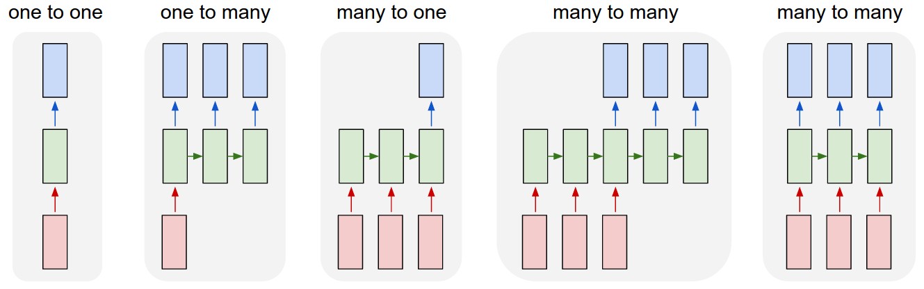
• seq2seq (seq2vec –> vec2seq): this includes aligned (NER) or unaligned (MT) tasks. Usually seq2seq is referring to the unaligned tasks.

An example of different mappings for sequential tasks is given below from the famous Karpathy RNN post:

src

Sequence models for NLP encoder

As stated earlier, while context in CV is spatial, context in NLP is sequential. Hence, Encoders in CV uses ConvNets, while in NLP they need to use sequence models. Different ways to encoder context are possible:

• Bag-of-Words: which is just grouping of words, according to their index in the vocabulary, without any context or sequence/order information. Clearly this is the most naive way, however, the inference and trainig is fast since they use fully connected layers.

• Recurrent models: which is the natural choice to encode sequences. The most famous are LSTM and GRU, best explained in karpathy post. Being the SoTA for years in NLP, they always suffered the slowness of training and inference, being sequential processing pipelines, so they can’t really make use of parallelization in modern GPUs for example.

• ConvNet (CNN1D): ConvNets are the standard in 2D sparial images. In their core, they can hierarichally aggregate local features with enough stack of layers. The field of view of the convolutional kernel keeps expanding with depth, and hence can encode differnet chuncks of the sequence. They can also perform seq2seq tasks, as in convs2s. However, the main drawback is that the architecture depth now scales with the sequence length. Also, if some word has a relation to a far word in the context, it will not be captured or at the best case be captured in later layers.

Transformers were proposed by Google in 2017 to address the drawbacks of all the above models. Transformers are based on the idea of attention, previously used with recurrent models in Bahdanau and Luong for seq2seq models applied to NMT. The transformers paper takes attention to the limit, where it gets rid of LSTM altogether, and only uses attention mechanisms. At each level of encoding the sequence, A Query vector asks all the context Key word vectors about a certain feature. The encoded feature is an aggregation over all context words vectors Values, each contributing according to its Key vector similarity to the Query.

Since the model now is purely parallel, sequence information is lost. For that, a special Position feature is added to encode the order of the word in the sequence. Since position is another categorical variable, we need an Embedding to it (now you get the rule).

I like to think of transformers as a mixture of BoW+Attention+Position encoding. Transformers are best understood following this great post.

ImageNet moment for NLP - 2018

Computer vision community has exploited the Encoder-Decoder pattern, coupled with the Transfer Learning scheme, to build encoders on huge amount of data, ImageNet data, and fine-tune the trained encoders on other downstream tasks: classification, segmentation, detection,…etc.

ULMFiT

In 2018, ULMFiT followed the same paradigm, to perform transfer learning of a recurrent encoder on language modeling (LM) task, and fine tune it on other downstream tasks, like sentiment classificaiton.

ULMFiT used the encoder decoder as follows:

• Encoder (sent2vec): pre-trained on from Neural Language Model (NLM) using LSTM (next word prediction)
• Decoder (vec2cls): TL from NLM, and fine tune downstream (text classification)

GPT = UMLFiT + Transformer

ULMFiT was based on recurrent models (LSTM or GRU). Moreover, the focus in ULMFiT was to proof the idea of TL based on LM tasks, but no sharing of the pre-trained encoder happened (like the case in CV pre-trained nets like VGG, ResNet,…etc).

After the appearance of transformers, OpenAI took the idea of ULMFiT and applied it using transformers as the sequence encoder.

GPT-2

Just a bigger GPT-1

GPT-3

Again, bigger GPT-2, plus:

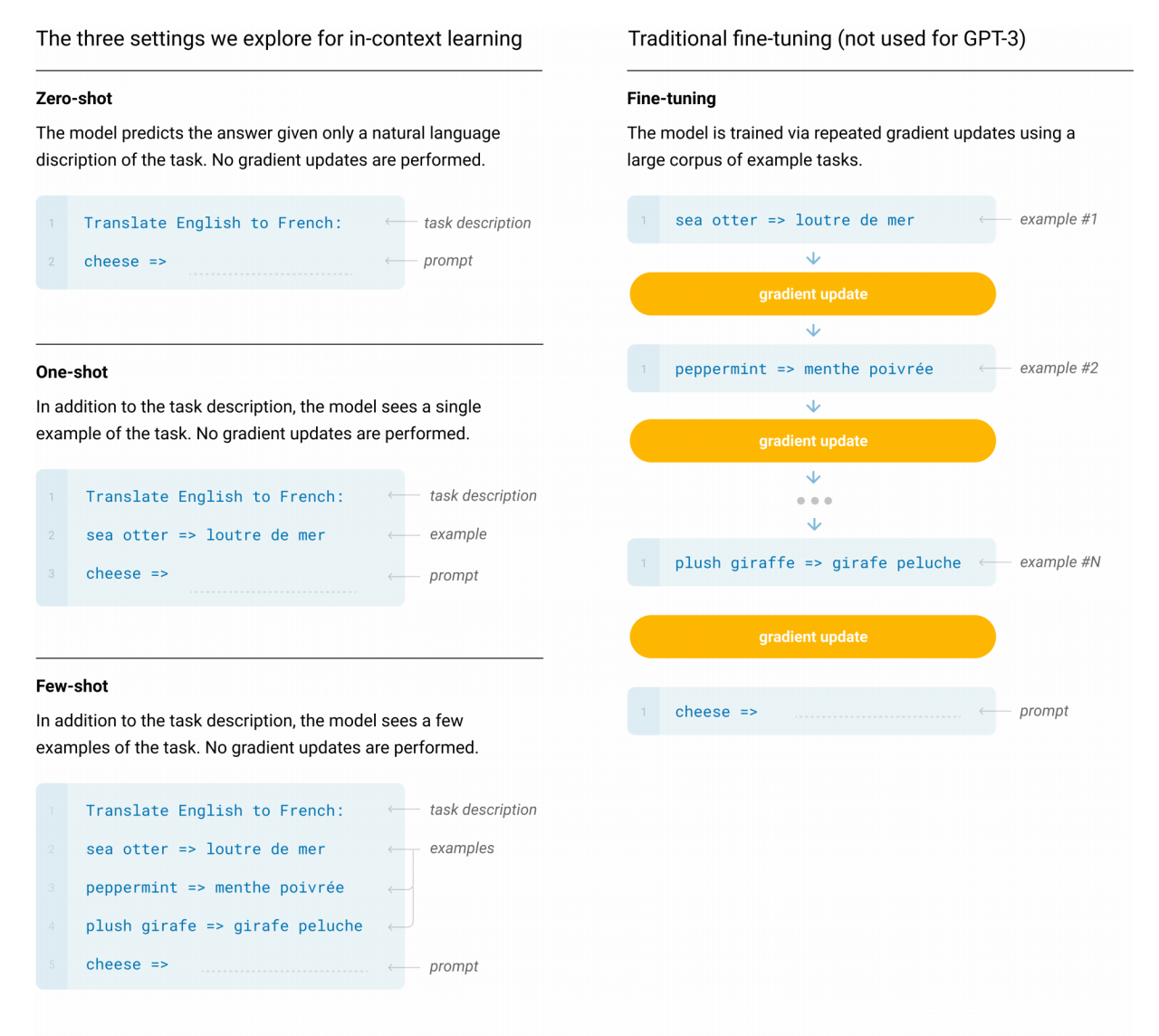
GPT-3 LM are Few-shot learners

In GPT-3, a gigantic model is trained only for language modeling. No fine tuning what so ever is done for downstream tasks. Three scenarios are defined in the paper: zer-shot, one-shot and few-shot learners. All of them involve no fine-tuning. With that said, GPT-3 is on-par or sometimes exceeding SoTA models with fine-tuning!

The way any task is performed in GPT-3 is by formulating it as a next-word LM task. First some “seed” or context is given, followed by a “prompt” or a question we ask the model. The model has seen almost eveything on the internet (this is true, as one of its training data, along with others, is Common Crawl dataset, which is crawl of internet text at a point of time in 2019!). Because of that, almost any question can answered. Same as you type some search query to Google, it’s probable that you get an answer in the first few links. Given the gigantic model size, it is easy to “memorize” big training data in its huge parameters, then query them when needed to give an answer. This idea was mentioned in this nice review of the paper.

src

BERT

BERT is a combination of all the preceeding efforts. It imports the following ideas from the following papers:

• ULMFiT –> TL using LM
• GPT –> Using transformers
• ELMo –> Bi-directional context

With the following differences:

src

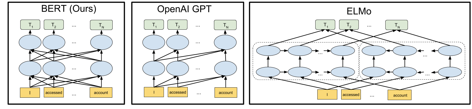
Truely Bi-directional

GPT LM models work in one direction: left-to-right (for English). For LM task, sometimes, the context is best guessed by looking on the next words, in addition to the preceeding words. We do that while reading. Since we have the whole sequence at hand, it’s ok to give the model access to the words before and after the missing word to be guessed.

ELMo models uses BiLSTM, so it encodes both directional contexts. However, if you look closely, every model have access to one direction at a time. We get a representation from each direction, then concatenate them. There’s no evidence why we should concatenate them, but there’s nothing else to do.

Given the following sequence: [w_1, w_2, …, w_x-1, w_x, w_x+1,…w_N], we want to guess what word w_x s, given [w_1, w_2,….w_x-1] AND [ w_x+1,…w_N]: $p(w_x|w_1, w_2, …, w_x-1, w_x+1,…w_N)$.

But BiLSTM does the following: 1- Get $p_1(w_x|w_1, w_2, …, w_x-1)$ 2- Get $p_2(w_x|w_x+1, w_x+2…w_N)$ 3- “Somehow” merge $p_1$ and $p_2$, which is by concatenating both represenations.

Auto Regressive (AR) vs Auto-Encoder (AE) Language Models

Next word prediction is a form of Auto-regressive language models. Even if this is in both directions like ELMo, it still an AR model.

The case of CBOW task in word2vec training is another form of LM, where a given word is predicted from all context words at once, regardless of direction. This is called Auto-encoder language model.

Masked LM (MLM)

To encode both directions using AE LM, BERT feeds to the transformer a sequence, with one or more words missing ([MASK]) and asks the model to decode the complete sequence by filling the missing words. More than one word could be missing from a sentence, where in BERT around 15% could be missing.

Next-sentence prediction

Another task, which is somehow similar to the skip gram with negarive sampling (SGNS) task of word2vec, is to feed two sentences, and ask the model if the first one can be the next one to the first.

Sub-word Embedding and OOV issue

Word level Embeddings suffer an issue called Out-Of-Vocabulary (OOV). Words have different morphologies (capitalized, prefix, suffix,…etc). Listing all different morpholoies is hard. This leads to sometimes encountering a word that has no entry in the table. To address this, some models work at the sub-word levels, to the lowest representation, which is the char level (the word as a sequence of chars). In this case, no OOV is possible, since the Embeddings happens at the char level, which has much less morphologies, and can all be listed. Another advantage of ELMo is using a mix of char level and word level models, called the sub-word level, which reduces the OOV. Since ELMo uses a sequence model (BiLSTM), it’s no issue to encode the word as a sequence of chars.

BERT uses sub-word representations. In sub-word level representation, first all characters have entries in the table. Followed by the sub-words, followed by the complete words. If a word is found as is, then it’s vector is used. If not, first we try to divide it into sub-words that are in the table, if not, we define it as sequence of characters.

src

BERT versions

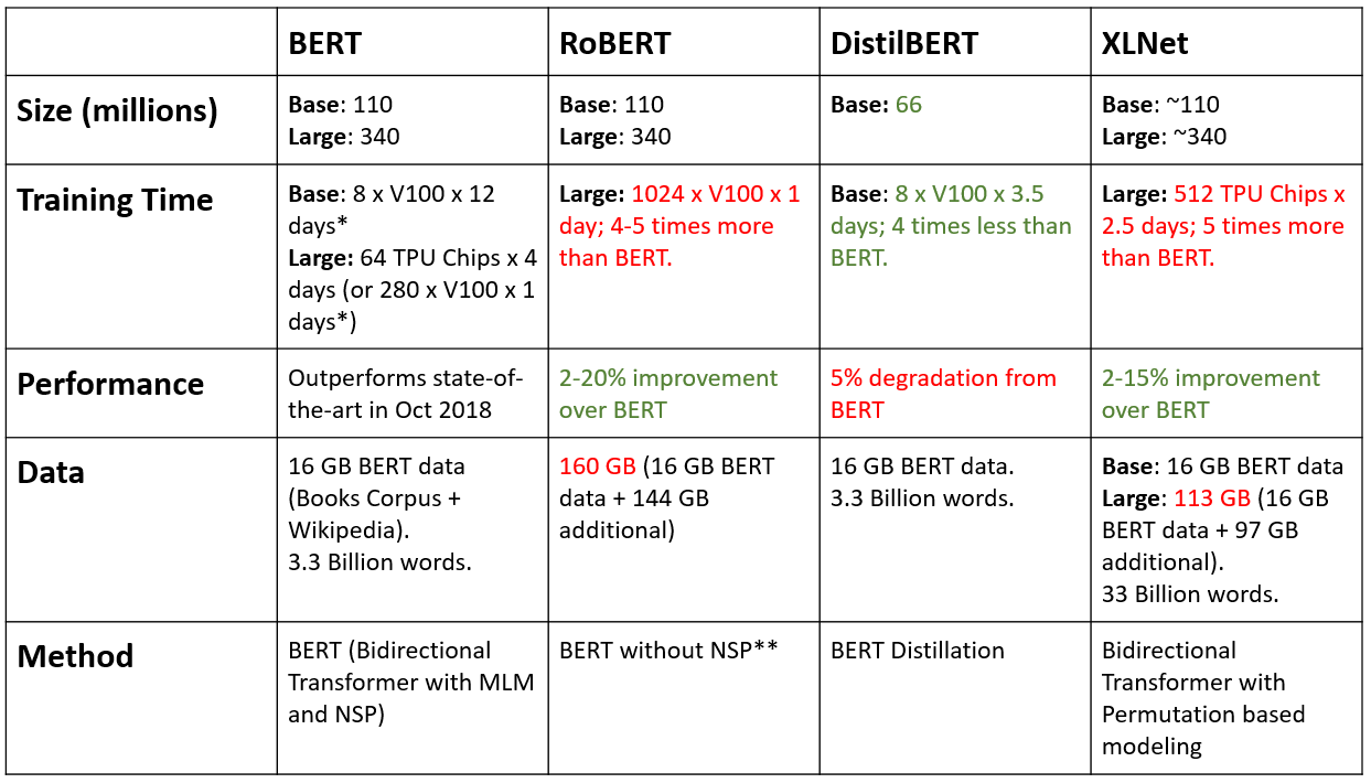
BERT comes with two versions: BERT_base (110M params) and BERT_large (340M params).

BERT-like

More models start to follow BERT, improving some parts, and doing some engineering tricks. In ALBERT, some tricks like sharing parameters across layers, and projecting the embeddings to a lower dimensional space, enables to have 18x smaller model than BERT large. Also, RoBERTa by FaceBook, removes completely the next-sentence prediction, and trains on larger (160GB) dataset.

XLNet

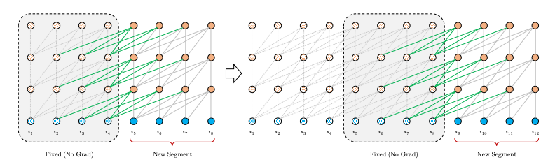
Transformer-XL = Recurrent Trasnformers

The traditional Transformer networks uses Positional encoding to encode sequence order. While training, the text is segmented into chunck of words called segments. Within a segment, the positional encoding is valid, while across the segments, no context is preserved. This means that the transformers will suffer in longer contexts spanning many segments. This was not the case (at least conceptually) with LSTM, where the state is kept over the segments.

To address this Xtra-Long Transformers were developed by GoogleBrain, adding recurrence over transformer encoded vectors, such that context is kept across segments.

src

What’s wrong with BERT

BERT uses AE LM for MLM task. This means that, if we have more than one token to predict ([MASK]), all of them can be predicted in parallel, without waiting to see the result of each others. On one hand, this is fast, but on the other hand, it can lead to wrong decoding if the masked words depend on each others.

In AR models, decoding is sequential, meaning, a decoded word always look to its left, adn decode a word, then this is given to the next to decode, and so on.

A nice example is given in the XLNet paper, for the case of decoding the following: [MASK], [MASK], is, a city ==> New, York, is, a, city. BERT AE LM will decode both words independently, leading to possibly invalid combinations. While an AR would decode them sequentially, so both words will depends on each others. However, AR LM are uni-directional.

Permutations LM (PLM)

To address this, XLNet uses a new task called Permutations LM. It follows the AE decoding way when decoding single MASK token, where like in CBOW, the central word is predicted given ALL context words, before or after. Unlike BERT MLM, the PLM generates ALL possible permutations of each word given the others. For each permutation, the masked word is predicted from the context (before or after). When a word is predicted, the next permutation will be generated based on that prediction.

src

The permutations prediction model will depend on how we factorize the sentence. In AR, the sentence is factorized always left to right. In PLM, we can have different factorizations, depending we want to predict the word from which context words. The example below from the XLNet paper, always token x3 is to be predicted. However, according to the factorization sequence, x3 will only be predicted from the left context. It doesnt mean this is the actual order (see the example 2-4-3-1, where x3 is [MASK], while others are not), but it just mean this is the context ot use to predict the word, e.g. x3.

src

BERT vs XLNet

BERT = Trans + MLM XLNet = XLTrans + PLM

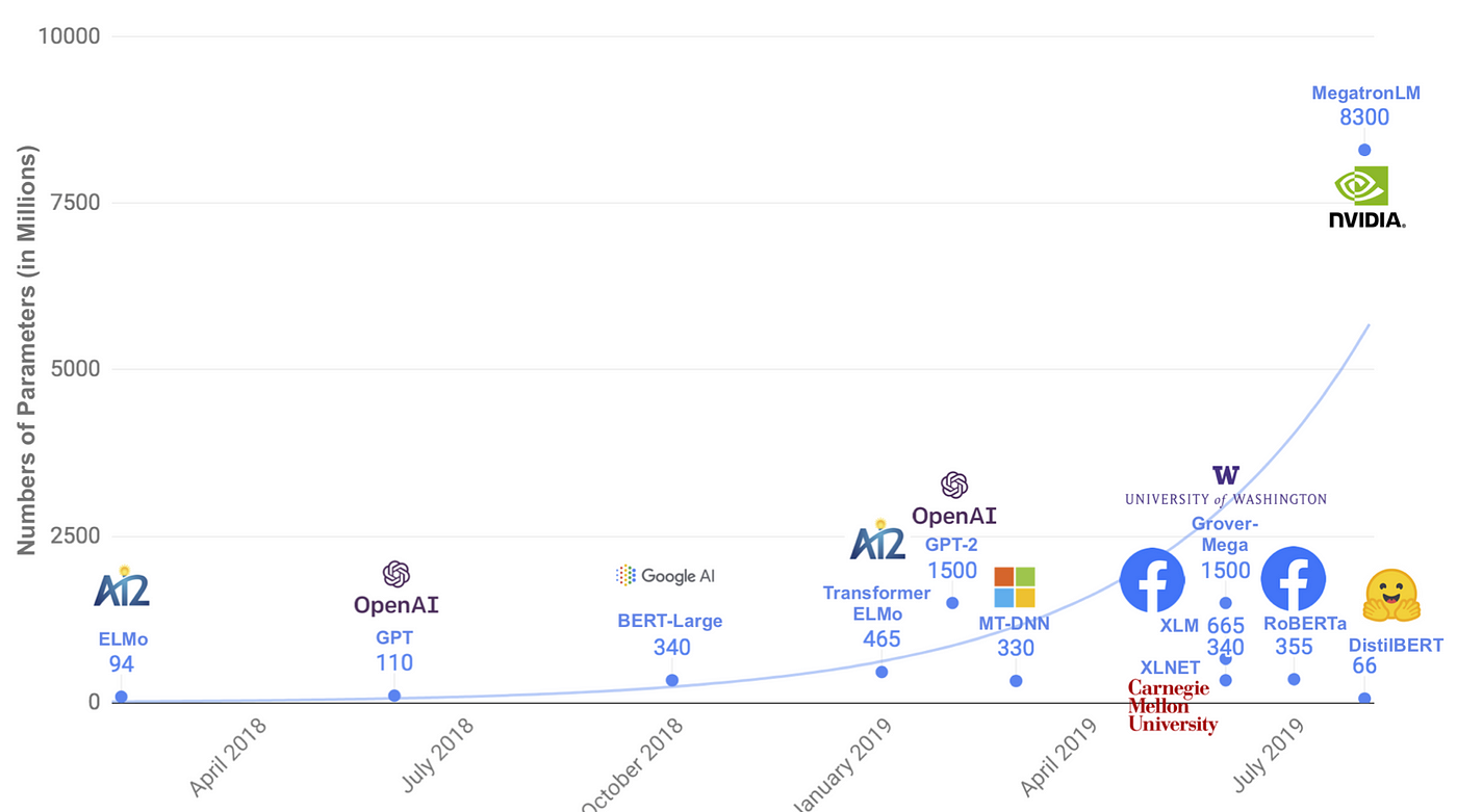
Cost of Gignatic TL models

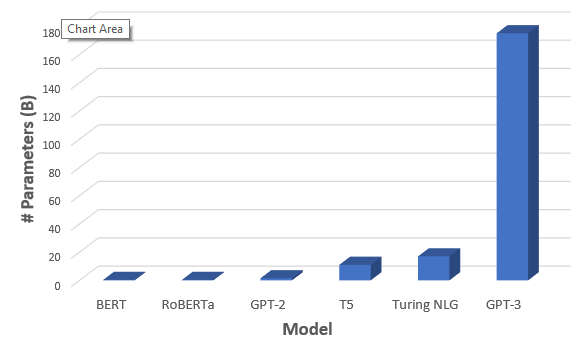
BERT and XLNet are around 110M params for the small model, while 340M for the big versions.

GPT-3 size reaches 175B parameters, with around 700GB disk space model!

The cost of training such models is huge:

This was mentioned in this XLNet paper review

Also, if an error happened during training, it’s hard to reset! In GPT-3, they discovered a “contamination”, where one dataset was very similar to some of the test data. However, they just reported that in the paper, as it was not possible to restart!

Given the huge models sizes, it is almost impossible to train from scratch (at least for individuals, small and medium sized entities or companies). This makes it hard to train also for languages other than English (Arabic, Chinese,…etc).

DistilBERT

One possible way is to “distill” the knowledge out of the large models, and train a smaller one, an idea in a paper by Hinton, 2015:

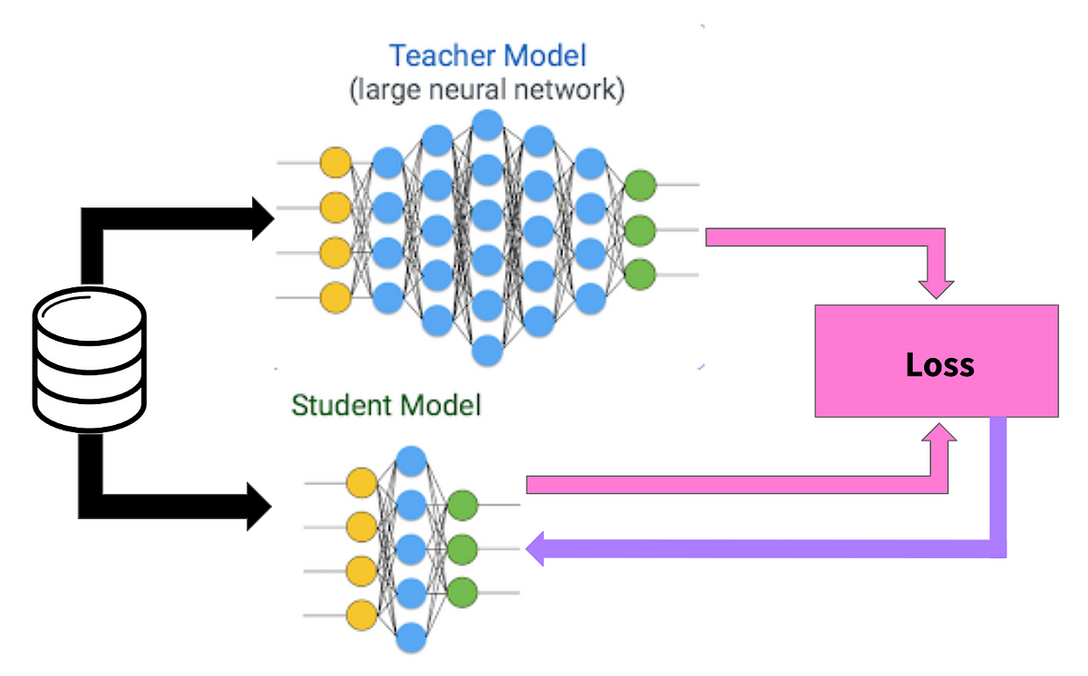
And so DistilBERT was born. I quote from the paper abstract: “we leverage knowledge distillation during the pre-training phase and show that it is possible to reduce the size of a BERT model by 40%, while retaining 97% of its language understanding capabilities and being 60% faster.”

src

src

What’s next?

Unsupervised

With the release of GPT-3, completely unsupervised on downstream tasks, gives high promises to unsupervised text models. So far, these models are not best at reasoning.

Reasoning and RL

The step towards transfer learning was huge in NLP. However, the SoTA models still seem far away from human reasoning (more towards AGI than ANI). May be the next frontier is to focus more on Reinforcement Learning (RL) methods, to learn from interactions. There are already a lot of attempts.

Smaller

Gignatic models like GPT and BERT makes it impractical for small groups to train from scratch. The need to make them smaller makes the field of NLP models compression important, like in DistilBERT

Conclusion

We have seen how the symbolic nature of language tasks adds an extra encoding step (Embedding) on the basic data constituents; say words. This was not needed for continous or numerical data (like pixels). We’ve seen that the problem extends to other domains like structured DL. This leads to the first TL attempt, at the word level models, or word Embeddings. The past few has witnessed a tremenedous growth in TL in NLP, where a similar path to CV domain has been followed. As we’ve seen, researchers begin to recognize the importance of having sentence level TL, same as in CV we embed the whole image, not pixels. This lead to SoTA architectures, that build on each others; ULMFiT, ELMo, GPT, BERT, XLNet,…etc.

References:

Appologies for the unorganized and non-formal references, but all sources are hyper-linked in the text above.

https://thegradient.pub/nlp-imagenet/ https://www.deeplearningbook.org/ https://www.manning.com/books/deep-learning-with-python http://jalammar.github.io/illustrated-word2vec/ https://www.tensorflow.org/tutorials/structured_data/feature_columns http://www.jmlr.org/papers/volume3/bengio03a/bengio03a.pdf https://nlp.stanford.edu/projects/glove/ http://cs224n.stanford.edu/ https://allennlp.org/elmo http://jalammar.github.io/illustrated-bert/ https://arxiv.org/abs/1801.06146 https://papers.nips.cc/paper/5346-sequence-to-sequence-learning-with-neural-networks.pdf http://karpathy.github.io/2015/05/21/rnn-effectiveness/ https://arxiv.org/abs/1705.03122 https://arxiv.org/abs/1706.03762 https://arxiv.org/abs/1508.04025 https://arxiv.org/abs/1409.0473 http://jalammar.github.io/illustrated-transformer/ https://openai.com/blog/better-language-models/ https://arxiv.org/abs/2005.14165 https://arxiv.org/abs/1810.04805 https://arxiv.org/abs/1909.11942 https://arxiv.org/abs/1907.11692 https://arxiv.org/abs/1906.08237 https://www.youtube.com/watch?v=H5vpBCLo74U https://arxiv.org/abs/1503.02531 https://arxiv.org/abs/1910.01108 https://github.com/adityathakker/awesome-rl-nlp